(Você pode ler esse post em português)
GDP (Gross Domestic Product) is a measure that represents the sum in monetary values of all final goods and services produced in a given region [1]. In Brazil, the value is normally released every quarter of the year. Next, I will present a methodology for forecasting the GDP value for the next quarter using Data Science techniques. The task can be viewed as a time series forecasting problem. To organize the reasoning, I will follow the steps of the KDD process (Knowledge Discovery in Databases) [2]. The code was built in Python, using the most widespread libraries of this language in data science (pandas, numpy, scikit-learn).
Selection
The original data was extracted from IBGE (Portuguese acronym for the Brazilian Institute of Geography and Statistics) [3]. The database contains the historical series of the GDP variation per semester, from the beginning of 1996 to the end of 2019. The extraction was done by downloading a file in CSV format. The study used data from the last 24 years for this period to represent a more stable range of variation in Brazilian GDP, coinciding with the stabilization of the current currency, in 1994. The prediction of future values for a time series achieves results closer to reality when current patterns do not differ substantially from historical values. Using older data makes certain distortions possible. Below, a figure of the referred data source with the time series plot.
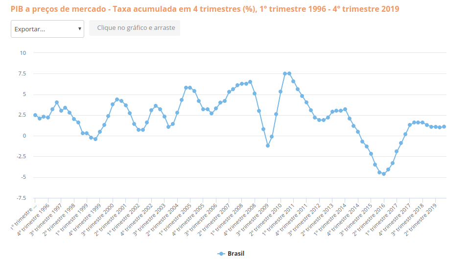 Fig. 1 - GDP variation quartely variation (1996 to 2019)
Preprocessing
Since we have a one-dimensional time series without missing data, it was not necessary to perform pre-processing operations. However, I will include in this section the analysis of the autocorrelation function (ACF). Autocorrelation refers to the correlation of a signal with its delayed values [4]. In other words, the analysis of this behavior allows us to understand how many past values of a time series influence the future values. The following image shows the autocorrelation function plot for the studied time series.
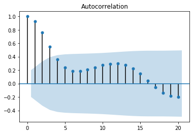
Fig. 2 - Time series autocorrelation function
This chart tells us how many past values significantly impact each point in the series. We can extract this information by looking at how many peaks are placed outside the central cone (painted in blue). Thus, we can conclude that, in general, it will be possible to predict the future values of the series by observing at least the four immediately previous values. Besides, the almost regular variation between the positive and negative peaks indicates a short seasonality in the series.
1
2
3
4
5
6
7
8
9
10
11
12
13
import pandas as pd
import numpy as np
import matplotlib.pyplot as plt
from pandas import DataFrame
from statsmodels.graphics.tsaplots import plot_acf
from statsmodels.tsa.seasonal import seasonal_decompose
from sklearn.model_selection import train_test_split
from sklearn import linear_model
from sklearn.metrics import mean_squared_error, r2_score, mean_absolute_error

file_name = '20200310012841.csv'
df_timeseries = pd.read_csv(file_name)
plot_acf(df_timeseries['gdp'])
Transformation
To predict time series in a standard machine learning modeling, the database must be in a matrix format: a set of n input vectors, usually multidimensional. Thus, a certain amount of delayed values may be used to create each of the input vectors. Consider, for example, a time series formed by the integers 4, 7, 5, 8, 10, 1, 0, 8, 3, 4, 2, 6. To transform this series into a dataset for supervised learning, we define the number of lags and build the n vectors labeled with the expected values. For example, with lags = 4, the previous time series becomes the following dataset (desired values in italic):
4, 7, 5, 8, 10
7, 5, 8, 10, 1
5, 8, 10, 1, 0
8, 10, 1, 0, 8
10, 1, 0, 8, 3
1, 0, 8, 3, 4
0, 8, 3, 4, 2
8, 3, 4, 2, 6
How many lagged values should we use? The plot of the autocorrelation function can give us a direction. In the quarterly GDP problem, we noted earlier that 4 is the number of past values that significantly influence the points in the series. This amount can be used as a starting point. Sometimes more detailed experimentation or study of the data is necessary to reach the optimal value. In a process driven by trial and error, I realized that running a few experiments that 8 is a good option. In this case, I am using the GDP variations of the last 8 quarters (two years) to forecast the value for the next quarter.
1
2
3
4
5
6
df = DataFrame()
df['t'] = df_timeseries['gdp']
lags = 8
for l in range(1, lags+1):
    df['t-'+str(l)] = df['t'].shift(l)
df = df.iloc[lags:]
Data Mining
In the data mining step, the goal is to use some model or algorithm of statistics or machine learning to obtain predictions. In this study, the model used was the well known linear regression. As usual, the dataset was partitioned between training (60%) and testing (40%). The determination coefficient (R2) in the test database was 96%. This metric is the proportion of the variance of the target variable that is explained by the input variables (the lagged values) [5]. Considering that its maximum value is 100%, the achieved results seem adequate. For a graphical analysis of the predictions, the figures below show the dispersion plots (blue for training and orange for testing) and the comparison between real (blue) and predicted (orange) values in the training and test datasets, respectively.
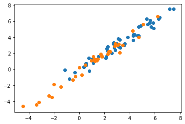
Fig. 3 - Dispersion plot between expected and predicted values
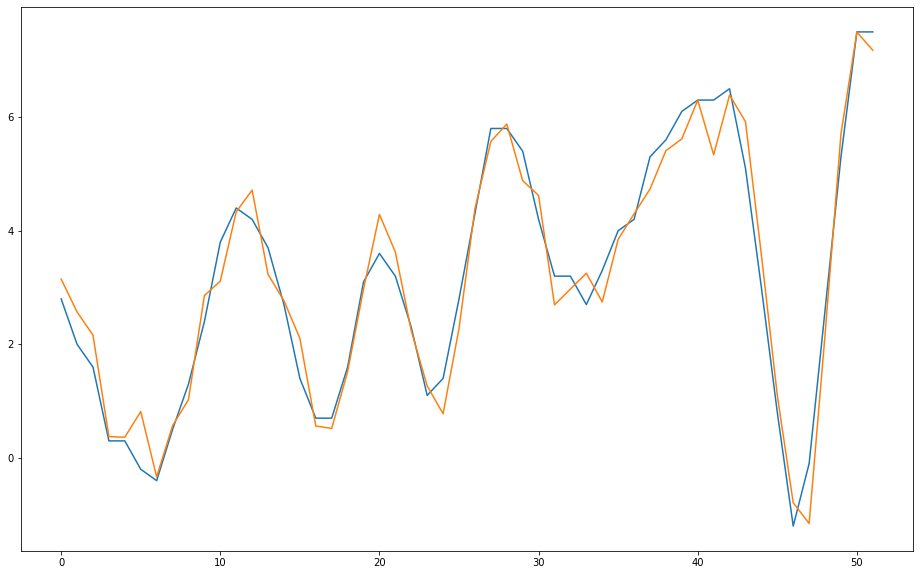 Fig. 4 - Expected (blue) and predicted (orange) values in the training dataset
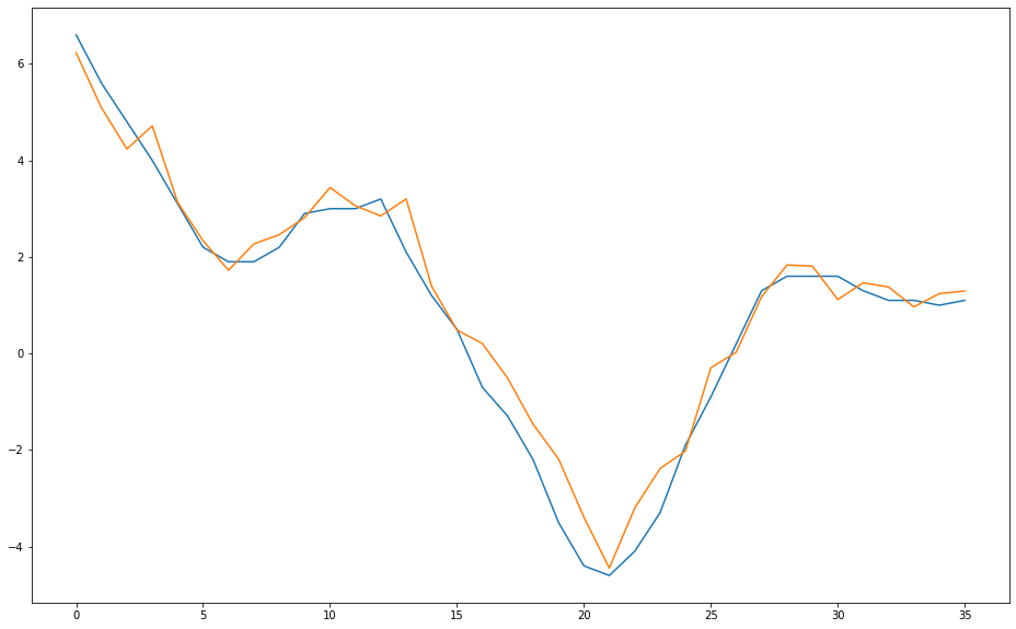 Fig. 5 - Expected (blue) and predicted (orange) values in the test dataset
1
2
3
4
5
6
7
8
9
10
11
12
13
14
15
16
17
18
19
20
21
22
23
24
25
26
27
28
29
30
31
X = df.iloc[:, 1:df.shape[1]]
y = df.iloc[:, 0]

X_train, X_test, y_train, y_test = train_test_split(X, y, test_size=0.4, shuffle=False)

regr = linear_model.LinearRegression()
regr.fit(X_train, y_train)
y_pred_train = regr.predict(X_train)
y_pred = regr.predict(X_test)

print('Coefficients: \n', regr.coef_)
print(y_test.shape)
print('Mean squared error (TRAIN): %.2f' % mean_squared_error(y_train, y_pred_train))
print('Mean absolute error (TRAIN): %.2f' % mean_absolute_error(y_train, y_pred_train))
print('Coefficient of determination (TRAIN): %.2f' % r2_score(y_train, y_pred_train))
print('Mean squared error (TEST): %.2f' % mean_squared_error(y_test, y_pred))
print('Mean absolute error (TEST): %.2f' % mean_absolute_error(y_test, y_pred))
print('Coefficient of determination (TEST): %.2f' % r2_score(y_test, y_pred))

plt.scatter(y_pred_train, y_train)
plt.scatter(y_pred, y_test)

fig = plt.figure(figsize=(16, 10))
ax = plt.axes()
ax.plot(y_train.to_numpy())
ax.plot(y_pred_train)

fig = plt.figure(figsize=(16, 10))
ax = plt.axes()
ax.plot(y_test.to_numpy())
ax.plot(y_pred)
Interpretation
Through the presented methodology and the analysis of the achieved results, it is possible to conclude that the linear regression from lagged values is a good model for forecasting the quarterly variation of the Brazilian GDP. Thus, if the behavior of the time series does not vary substantially concerning its history, it is feasible to anticipate the variation of the quarterly GDP with some advance. Two points deserve discussion:
It is necessary to discuss with experts in the field if this type of forecast is useful in a practical way. The forecast horizon may need to be changed. In this case, the model could predict the change in GDP over the next six months or even the next year. Several approaches can be taken to achieve this. Perhaps some of them should be discussed in future publications.
It should be noted that the studied time series in this article is hugely influenced by exogenous variables (variables external to the series, such as economic indices, world market behavior, epidemics, etc.). A more reliable model must take at least some of these variables into account. However, the methodology presented here represents a didactic starting point for further analysis.
Source code: https://github.com/andersontenorio/brazilgdpforecasting
REFERENCES
[1] https://en.wikipedia.org/wiki/Gross_domestic_product
[4] https://en.wikipedia.org/wiki/Autocorrelation
[5] https://en.wikipedia.org/wiki/Coefficient_of_determination